Introduction to fitting age-specific space-for-time mark-recapture models

1. Introduction

The space4time package is used to fit an age-specific space-for-time mark-recapture model. This vignette provides the basic details on formatting data for the models and fitting the models. Load the space4time package by running

library(space4time)

To briefly describe the purpose of these models and when then would be useful, space-for-time substitutions are frequently used in mark-recapture models for animals that migrate along a fixed path. Instead of repeated observations over time, there are observations of individuals as they pass fixed stations or sites. This is not a perfect substitution, because the amount of time it takes individuals to move between sites can vary. This model incorporates time and individual ageclass into the space-for-time framework. Here, ageclasses are with respect to time, so they are ages rather than stages like “juvenile” or “adult”.

The development of this model was motivated by migrating juvenile steelhead, which can be tagged as they exit rearing habitat. They can wait up to a few years before migrating out to the ocean, passing by observation stations (i.e. antennae that detect individuals with passive integrated transponder tags). Their survival and movement depends on age, so we made this model age-specific. However, ages are only measured for a subset of individuals, so we use a sub-model for age and then incorporate the uncertainty in age assignment into the mark-recapture likelihood.

The mark-recapture likelihood is the product of the likelihood of the observed data, where the probability that an individual transitions from site j to site k given that it passed site j at time s and during age a1 is $\Theta_{j,k,s,a_1,a_2,r,g}$. The probability that this individual is observed at site k is $p_{j,k,t,a_1,a_2,r,g}$. The mark-recapture likelihood incorporates the probability age assignments ($\pi_{i,s,a}$) for each individual $i$, where the mark-recapture probabilities are weighted over the probability age assignments (i.e. $\sum_{a1}{\Theta_{j,k,s,a_1,a_2,r,g} * \pi_{i,s,a1}}$). A full description of the likelihood and model implementation is given in (forthcoming manuscript).

There are two additional indices for the $Theta$ and $p$ arrays: initial release group $r$ and group $g$. The initial release group is where individuals were first captured (or observed). The group $g$ allows for individual covariates to be included. The implementation here uses formulas for the $Theta$ and $p$ parameters [add link to covariate vignette]. The formula for detection probability $p$ is:

$$logit(p) = X\beta$$ where $X$ is a design matrix of data and $\beta$ are parameters.

The formula for $\Theta$ uses intermediary parameters for conditional transition rates ($\theta$), which are the probability that an individual transitions from site j to k during time t given that it did not transition from site j to k in the previous time period. This accounts for individuals that holdover between sites for a time period or more.

$$\Theta_{j,k,s,a_1,a_2,r,g} = \theta_{j,k,s,a_1,a_2,r,g}\prod^{a2-1}_{v=a_1}{\theta_{j,k,s,a_1,v,r,g}}$$

$$logit(\theta_{j,k,s,a_1,a_2,r,g}) = Y\gamma$$ where $Y$ is a design matrix of data and $\gamma$ are parameters.

2. Data

To demonstrate the format that data need to be in to be read, data is simulated using a built-in function

set.seed(1)
sim.dat <- sim_simple_s4t_ch(N = 800)

s4t_ch <- sim.dat$s4t_ch

This returns a capture history object (s4t_ch). The key pieces of data of interest are the capture history, individual auxiliary data, and site configuration.

a. The capture history data:

Each row represents an observation or capture instance. There must be four columns, described in the table below.

Required columns:

Column	Description
id	Uniquely identifier
site	Observed site name
time	Observation time period. Integer or date (converted to year)
removed	Whether individuals were removed at this point

Example first 6 rows:

id	site	time	removed
1	1	2	FALSE
1	2	3	FALSE
2	1	1	FALSE
2	2	1	FALSE
3	1	1	FALSE
3	2	2	FALSE

b. Individual auxiliary data

There must be example one row for each individual. There are three required columns and any extra columns can be included. Order of columns does not matter.

Required columns:

Column	Description
id	Uniquely identifying code or number
obs_time	Observed time period when auxiliary data were collected
ageclass	Integer ageclass

Example first 6 rows:

id	obs_time	FL	ageclass
1	2	-2.8	NA
2	1	-1.5	2
3	1	0.9	NA
4	1	4.9	3
5	2	-3.6	1
6	1	4.8	3

c. Site configuration

The site configuration is an object nested within the s4t_ch object. A summary of the site configuration (s4t_config object) can be shown by printing the object:

#> Site and age transition configuration object
#> 
#> There are N = 3 with N = 1 sites with holdovers
#> 
#> Sites: 1, 2, 3
#> 
#> Sites with holdovers: 1
#> 
#> Site -> site:
#> 1 -> 2
#> 2 -> 3
#> 3 -> 
#> 
#> Age range per site:
#> 1: 1-3
#> 2: 1-3
#> 3: 1-3

There are three sites, where one of the sites has holdovers, meaning that individuals can wait a time period or more between sites. The sites are named 1, 2, and 3. The site with holdovers is site 1, meaning that after individuals pass site 1, they can wait a time period or more before transitioning to the next site (site 2). The order and arrangement of the sites is shown by Site -> site, and the possible age ranges that individuals can be in each site are shown by Age range per site.

This object was generated using the following:

ex_config <- linear_s4t_config(sites_names = 1:3, # vector of site names
                               holdover_sites = 1,# which site (or sites) do 
                               # individuals holdover before continuing to the next site
                               min_a = c(1,1,1), # for each site, the minimum possible age
                               max_a = c(3,3,3)) # for each site, the maximum possible age

The linear_s4t_config() function is used to create these s4t_config objects. For more complex site configurations, simplebranch_s4t_config() or s4t_config() can be used.

d. Creating the s4t_ch object

The s4t_ch object can be created using the elements from above:

ex_ch <- s4t_ch(ch_df = ch_df,
                aux_age_df = aux_df,
                s4t_config = ex_config)

4. Fit ageclass model

Prior to fitting the full model, the sub-model for ageclass can be fit separately to select the best fitting model for ageclass. The fit_ageclass function uses ordinal regression with the observed age-class of individuals as a response. Covariates (which must be included in the individual auxiliary data when creating the s4t_ch object) can be included, using standard formula notation. We use the logit link and transitions between age groups are sequential. The threshold between each age group was estimated as parameters of the model.

age_m1 <- fit_ageclass(age_formula = ~ 1,s4t_ch = s4t_ch)

age_m2 <- fit_ageclass(age_formula = ~ FL,s4t_ch = s4t_ch)

# note that obs_time is treated as a factor (see fit_ageclass documentation)
age_m3 <- fit_ageclass(age_formula = ~ FL + obs_time,s4t_ch = s4t_ch)

The models can be compared using AIC:

AIC(age_m1, 
    age_m2, 
    age_m3)
#>        df      AIC
#> age_m1  2 471.4208
#> age_m2  3 229.0453
#> age_m3  4 229.6865

The top model by AIC is age_m2.

5. Fit space-for-time mark-recapture model

There are two options for fitting space-for-time mark-recapture models, implementations using Bayesian (fit_s4t_cjs_rstan) and maximum likelihood (fit_s4t_cjs_ml) methods. As of now, the Bayesian implementation is faster.

For the purposes of this example, the number of chains is set to 2 (recommend 3), the number of warmup iteration is 200 (recommend at least 500), and the number of total iterations is 600 (recommend at least 500 over the number of warmups).

The first three arguments are the formulas for detection probability (p), conditional transition rates (theta), and ageclass. The formulas allow for symbolic representation of the sub-models.

The formula for p below is ~ t, which represents detection probability varying by the time individuals pass sites. There is only one site (site 2) where detection probability is estimated, because detection is not estimated at the first site or last site (fixed to 1 at the last site because it is not separable from transition rates). If there were multiple sites where detection probability was estimated, the equivalent formula would be ~ t * k, which represents a different detection probability at each site at each time period. A table showing the meaning of each variable (j, k, s, t, r, g, a1, and a2) is shown below.

The formula for theta below is ~ a1 * a2 * s * j, which is the fully saturated model for this scenario with different transition probabilities for each combination of age, time, and site. The transition probabilities for individuals from site j to site k are conditioned on individuals not transitioning to site k in the previous time period. This is the fully saturated model for theta because there are no groups and because there is only one initial release site (site 1). If there were more than one initial release site, the full saturated model would be ~ a1 * a2 * s * j * r.

The argument fixed_age == TRUE allows for the ageclass model to be fit separately and the output fed into the mark-recapture model. The output is the estimated probabilities that individuals belong to each ageclass. The mark-recapture model uses the probability age assignments to integrate over the uncertainty in age.

Variable	Description
j	Release site
k	Recapture site
s	Release time
t	Recapture time
r	Initial release group
g	Group (individual covariate)
a1	Age during time s (“release”)
a2	Age during time t (“recapture”)

m1 <- fit_s4t_cjs_rstan(
      p_formula = ~ t,
      theta_formula = ~ a1 * a2 * s * j,
      ageclass_formula = ~ FL,
      fixed_age = TRUE,
      s4t_ch = s4t_ch,
      chains = 2,
      warmup = 200,
      iter = 600
    )
#> 
#> SAMPLING FOR MODEL 's4t_cjs_fixedage_draft7' NOW (CHAIN 1).
#> Chain 1: 
#> Chain 1: Gradient evaluation took 0.000861 seconds
#> Chain 1: 1000 transitions using 10 leapfrog steps per transition would take 8.61 seconds.
#> Chain 1: Adjust your expectations accordingly!
#> Chain 1: 
#> Chain 1: 
#> Chain 1: Iteration:   1 / 600 [  0%]  (Warmup)
#> Chain 1: Iteration:  60 / 600 [ 10%]  (Warmup)
#> Chain 1: Iteration: 120 / 600 [ 20%]  (Warmup)
#> Chain 1: Iteration: 180 / 600 [ 30%]  (Warmup)
#> Chain 1: Iteration: 201 / 600 [ 33%]  (Sampling)
#> Chain 1: Iteration: 260 / 600 [ 43%]  (Sampling)
#> Chain 1: Iteration: 320 / 600 [ 53%]  (Sampling)
#> Chain 1: Iteration: 380 / 600 [ 63%]  (Sampling)
#> Chain 1: Iteration: 440 / 600 [ 73%]  (Sampling)
#> Chain 1: Iteration: 500 / 600 [ 83%]  (Sampling)
#> Chain 1: Iteration: 560 / 600 [ 93%]  (Sampling)
#> Chain 1: Iteration: 600 / 600 [100%]  (Sampling)
#> Chain 1: 
#> Chain 1:  Elapsed Time: 16.243 seconds (Warm-up)
#> Chain 1:                28.902 seconds (Sampling)
#> Chain 1:                45.145 seconds (Total)
#> Chain 1: 
#> 
#> SAMPLING FOR MODEL 's4t_cjs_fixedage_draft7' NOW (CHAIN 2).
#> Chain 2: 
#> Chain 2: Gradient evaluation took 0.000739 seconds
#> Chain 2: 1000 transitions using 10 leapfrog steps per transition would take 7.39 seconds.
#> Chain 2: Adjust your expectations accordingly!
#> Chain 2: 
#> Chain 2: 
#> Chain 2: Iteration:   1 / 600 [  0%]  (Warmup)
#> Chain 2: Iteration:  60 / 600 [ 10%]  (Warmup)
#> Chain 2: Iteration: 120 / 600 [ 20%]  (Warmup)
#> Chain 2: Iteration: 180 / 600 [ 30%]  (Warmup)
#> Chain 2: Iteration: 201 / 600 [ 33%]  (Sampling)
#> Chain 2: Iteration: 260 / 600 [ 43%]  (Sampling)
#> Chain 2: Iteration: 320 / 600 [ 53%]  (Sampling)
#> Chain 2: Iteration: 380 / 600 [ 63%]  (Sampling)
#> Chain 2: Iteration: 440 / 600 [ 73%]  (Sampling)
#> Chain 2: Iteration: 500 / 600 [ 83%]  (Sampling)
#> Chain 2: Iteration: 560 / 600 [ 93%]  (Sampling)
#> Chain 2: Iteration: 600 / 600 [100%]  (Sampling)
#> Chain 2: 
#> Chain 2:  Elapsed Time: 18.523 seconds (Warm-up)
#> Chain 2:                29.275 seconds (Sampling)
#> Chain 2:                47.798 seconds (Total)
#> Chain 2:

The results can be printed out. Check that the Rhat values are all below 1.1 (for proper convergence/mixing)

print(m1)
#> Inference for Stan model: s4t_cjs_fixedage_draft7.
#> 2 chains, each with iter=600; warmup=200; thin=1; 
#> post-warmup draws per chain=400, total post-warmup draws=800.
#> 
#>                    mean se_mean   sd  2.5%   25%   50%   75% 97.5% n_eff Rhat
#> theta_(Intercept) -1.60    0.01 0.25 -2.14 -1.76 -1.59 -1.43 -1.14   571 1.00
#> theta_a12         -1.75    0.02 0.54 -2.94 -2.08 -1.72 -1.35 -0.80   611 1.00
#> theta_a13         -1.15    0.02 0.54 -2.34 -1.46 -1.14 -0.78 -0.17   603 1.00
#> theta_a22          0.18    0.02 0.38 -0.53 -0.06  0.18  0.42  0.91   589 1.00
#> theta_a23          3.54    0.02 0.54  2.65  3.16  3.48  3.87  4.76   601 1.01
#> theta_s2          -0.58    0.02 0.41 -1.38 -0.82 -0.58 -0.32  0.18   550 1.00
#> theta_s3           0.87    0.01 0.36  0.11  0.63  0.86  1.10  1.54  1015 1.00
#> theta_s4          -0.21    0.02 0.58 -1.34 -0.60 -0.20  0.18  0.90   931 1.00
#> theta_j2           1.40    0.02 0.49  0.40  1.08  1.40  1.74  2.30   624 1.00
#> theta_a12:a22      0.96    0.03 0.64 -0.26  0.54  0.96  1.38  2.28   637 1.00
#> theta_a12:s2       0.02    0.05 0.94 -1.93 -0.59  0.11  0.66  1.78   328 1.00
#> theta_a13:s2       0.04    0.05 0.92 -1.86 -0.56  0.15  0.70  1.58   325 1.00
#> theta_a12:s3       0.68    0.04 1.00 -1.11 -0.01  0.57  1.27  2.91   685 1.00
#> theta_a22:s2       2.82    0.02 0.52  1.80  2.47  2.84  3.16  3.87   537 1.00
#> theta_a23:s2       0.28    0.05 0.94 -1.36 -0.37  0.19  0.86  2.45   298 1.00
#> theta_a12:j2      -1.28    0.05 1.05 -3.66 -1.93 -1.22 -0.57  0.57   519 1.00
#> theta_a13:j2      -3.70    0.02 0.61 -4.89 -4.13 -3.69 -3.28 -2.49   635 1.00
#> theta_s2:j2        1.52    0.03 0.73  0.06  1.07  1.53  2.02  2.94   529 1.00
#> theta_a12:a22:s2   0.43    0.05 0.95 -1.26 -0.25  0.39  1.03  2.36   362 1.00
#> theta_a12:s2:j2   -1.49    0.05 1.16 -3.60 -2.33 -1.54 -0.66  0.77   496 1.00
#> theta_a13:s2:j2    0.41    0.04 0.83 -1.25 -0.10  0.40  0.89  2.05   550 1.00
#> p_(Intercept)      2.63    0.04 0.75  1.38  2.09  2.55  3.09  4.37   349 1.00
#> p_t2              -1.49    0.04 0.77 -3.27 -1.95 -1.44 -0.92 -0.23   352 1.00
#> p_t3              -0.57    0.04 0.83 -2.31 -1.04 -0.55 -0.03  0.93   387 1.00
#> p_t4              -0.76    0.06 1.26 -2.99 -1.60 -0.83 -0.05  2.01   476 1.00
#> overall_surv[1]    0.91    0.00 0.04  0.83  0.89  0.92  0.94  0.97   710 1.00
#> overall_surv[2]    0.60    0.00 0.05  0.50  0.56  0.60  0.63  0.70   914 1.00
#> overall_surv[3]    0.69    0.00 0.06  0.58  0.65  0.68  0.72  0.80   829 1.00
#> overall_surv[4]    0.94    0.00 0.04  0.87  0.92  0.95  0.98  0.99   400 1.00
#> overall_surv[5]    0.80    0.00 0.05  0.71  0.77  0.80  0.83  0.89   747 1.00
#> overall_surv[6]    0.63    0.00 0.05  0.53  0.59  0.63  0.66  0.74   793 1.00
#> overall_surv[7]    0.45    0.00 0.11  0.25  0.38  0.44  0.53  0.67   860 1.00
#> overall_surv[8]    0.14    0.00 0.09  0.01  0.07  0.12  0.18  0.34   865 1.00
#> overall_surv[9]    0.19    0.00 0.04  0.11  0.16  0.18  0.21  0.28   854 1.00
#> overall_surv[10]   0.67    0.00 0.12  0.42  0.59  0.68  0.75  0.86   820 1.00
#> overall_surv[11]   0.65    0.00 0.06  0.54  0.61  0.65  0.69  0.77   888 1.00
#> overall_surv[12]   0.54    0.00 0.05  0.45  0.51  0.54  0.57  0.63   953 1.00
#> overall_surv[13]   0.37    0.00 0.06  0.26  0.33  0.37  0.41  0.48   867 1.00
#> overall_surv[14]   0.35    0.00 0.05  0.26  0.31  0.34  0.38  0.44   978 1.00
#> overall_surv[15]   0.16    0.00 0.07  0.06  0.12  0.15  0.20  0.31   917 1.00
#> cohort_surv[1]     0.17    0.00 0.03  0.10  0.15  0.17  0.19  0.24   571 1.00
#> cohort_surv[2]     0.17    0.00 0.04  0.10  0.14  0.16  0.19  0.25   767 1.00
#> cohort_surv[3]     0.57    0.00 0.05  0.49  0.54  0.57  0.61  0.67   777 1.01
#> cohort_surv[4]     0.10    0.00 0.03  0.05  0.08  0.10  0.12  0.17   959 1.00
#> cohort_surv[5]     0.49    0.00 0.05  0.40  0.46  0.49  0.53  0.59   861 1.00
#> cohort_surv[6]     0.69    0.00 0.06  0.58  0.65  0.68  0.72  0.80   829 1.00
#> cohort_surv[7]     0.11    0.00 0.03  0.05  0.08  0.10  0.13  0.17   893 1.00
#> cohort_surv[8]     0.62    0.00 0.05  0.52  0.59  0.62  0.65  0.72   949 1.00
#> cohort_surv[9]     0.22    0.00 0.04  0.15  0.19  0.22  0.24  0.31   728 1.00
#> cohort_surv[10]    0.62    0.00 0.05  0.51  0.58  0.62  0.65  0.72   881 1.00
#> cohort_surv[11]    0.18    0.00 0.04  0.12  0.16  0.18  0.21  0.26   885 1.01
#> cohort_surv[12]    0.63    0.00 0.05  0.53  0.59  0.63  0.66  0.74   793 1.00
#> cohort_surv[13]    0.45    0.00 0.11  0.25  0.38  0.44  0.53  0.67   860 1.00
#> cohort_surv[14]    0.14    0.00 0.09  0.01  0.07  0.12  0.18  0.34   865 1.00
#> cohort_surv[15]    0.19    0.00 0.04  0.11  0.16  0.18  0.21  0.28   854 1.00
#> cohort_surv[16]    0.67    0.00 0.12  0.42  0.59  0.68  0.75  0.86   820 1.00
#> cohort_surv[17]    0.65    0.00 0.06  0.54  0.61  0.65  0.69  0.77   888 1.00
#> cohort_surv[18]    0.54    0.00 0.05  0.45  0.51  0.54  0.57  0.63   953 1.00
#> cohort_surv[19]    0.37    0.00 0.06  0.26  0.33  0.37  0.41  0.48   867 1.00
#> cohort_surv[20]    0.35    0.00 0.05  0.26  0.31  0.34  0.38  0.44   978 1.00
#> cohort_surv[21]    0.16    0.00 0.07  0.06  0.12  0.15  0.20  0.31   917 1.00
#> 
#> Samples were drawn using NUTS(diag_e) at Mon Mar 16 17:00:57 2026.
#> For each parameter, n_eff is a crude measure of effective sample size,
#> and Rhat is the potential scale reduction factor on split chains (at 
#> convergence, Rhat=1).

Evaluate traceplots of each estimated parameter:

traceplot(m1,pars = "theta")

traceplot(m1,pars = "^p") # regular expressions for all parameters that start with "p"

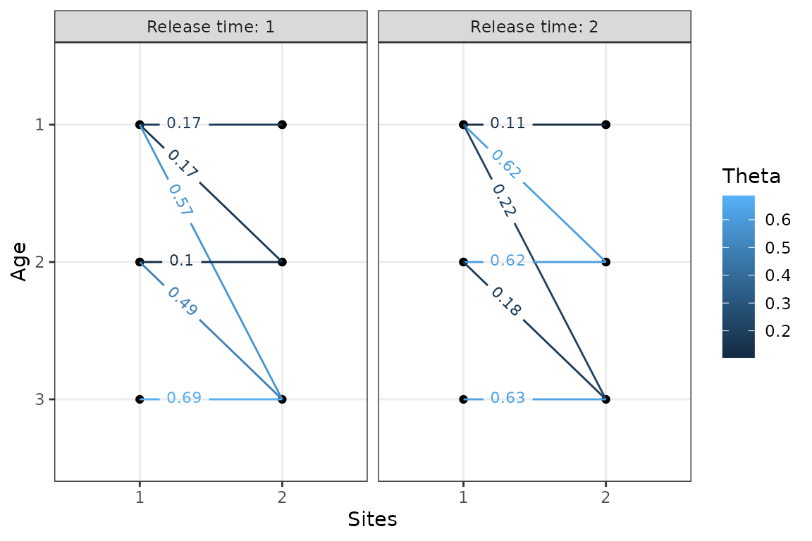
plotSurvival(m1)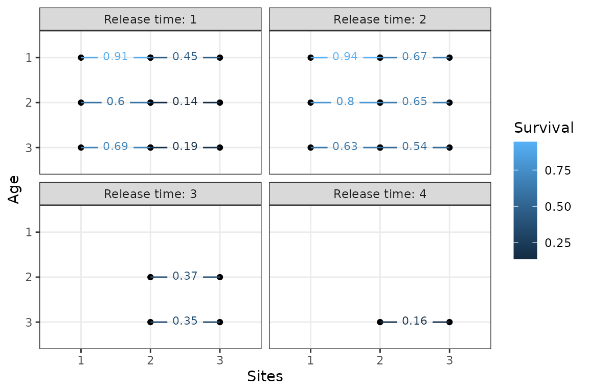

plotTransitions(m1,textsize = 3, j == 1) # only include transitions that start from site 1